Apr 20, 2023

Scaling Out to Apache Spark with Ibis

Jordan Volz

Over the past decade, Apache Spark has been a widely used data engine for distributed data processing and analytics. Teams that outgrew single-node data analysis have often flocked to Spark, as its interface was often leagues above what other distributed systems offered at the time. Additionally, Python users were courted with PySpark, which provided a Pythonic distributed interface and prevented them from having to learn Java or Scala. While this is sufficient for large workloads, the reality for Python users is that Spark is clumsy to work with locally on a laptop and can be expensive to use on a cluster. As a result, many Python users still develop locally in something like pandas, which is cheap and easy to use, and then rewrite code into PySpark for production work. This procedure of rewriting code in order to scale it from local to distributed adds a non-trivial amount of complexity and risk into data workflows. For many data teams, this is the status quo in 2023. But, what if there was a better way?

Why Ibis?

Ibis is an open source Python library that bills itself as “the flexibility of Python analytics with the scale and performance of modern SQL”. What does it do? Ibis allows users to define data operations in Python, using a familiar pandas-like syntax, which are then executed on a specified backend, such as BigQuery, Snowflake, or PySpark, among others. Under the covers, Ibis converts these Python operations into expressions compatible with backends, like SQL statements, that are then executed on the backend.

There are three things to love about how Ibis works:

1. Push compute to the backend to run natively in the specified engine.
2. Strategy for scaling data workloads
3. Protect your data team from vendor lock-in

First of all, by translating data operations into SQL statements, Ibis is able to push all the compute down into the backend so it runs natively in the specified engine. Ibis doesn’t try to perform operations on data itself, which provides a lot of efficiency and scalability (when needed). In fact, this compilation and pushdown strategy is very similar to another open source tool that is widely popular: dbt.

At the most basic level, dbt has two components: a compiler and a runner. Users write dbt code in their text editor of choice and then invoke dbt from the command line. dbt compiles all code into raw SQL and executes that code against the configured data warehouse.

Whereas dbt focuses mainly on allowing users to write SQL (1) and compiles it into SQL to execute it in their data warehouse, Ibis allows users to write Python and compiles it into SQL to execute on the specified backend.

Secondly, Ibis provides an excellent strategy for scaling data workloads. Once an Ibis workflow is written, users only need to connect to a different backend in order to change where the workflow runs. None of the workflow code needs to be modified. For example, a data practitioner can use Ibis to develop a workflow locally and run it on a local machine using a supported backend like MySQL, DuckDB, or even pandas, and then easily run it on a full dataset on a distributed platform like Snowflake, PySpark, or Trino. Gone are the days of rewriting code for your distributed data platform, and this represents an excellent way to supercharge your company’s development to production data workflows.

Since Ibis easily allows users to move workflows from one backend to another, this helps illuminate the third great aspect of Ibis: it helps protect your data team from vendor lock-in. We’ve all probably had the experience of participating in at least one database migration before and we know they’re painful. And, even though every database out there is ANSI-compliant, over time data teams are drawn into leveraging the non-compliant parts of the system. While this may alleviate some workload strains in the short term, the long-term effect is that data systems are difficult to migrate and require a large amount of query rewrites. These exercises end up being expensive for customers – either in human capital or real dollars paid to consultants who love to sit around and translate queries. Ibis paints a different picture: write workloads once, and run them anywhere.

Enough grandstanding, let’s see Ibis in action.

A Local Example

We’ll start by running Ibis on a small amount of data in a local example.  For this example, we’ll use the KKBox churn dataset from Kaggle, which you can freely download and load up into your storage layer of choice. This dataset has a lot of data from a music streaming service. For our use, we’ll be interested in aggregating the user_log dataset to create some new features which might be useful in downstream machine learning applications.

Even though we’ll only be using the user_logs dataset for this example, you might notice that this amounts to over 30GB of (CSV) data. This is nothing to sneeze at. If your local computer won’t handle data that large, feel free to quickly generate a workable sample. Linux or Mac users can use the following for that task:

head -n 100000 kkbox-churn-prediction-challenge/data/user_logs.csv > 
kkbox-churn-prediction-challenge/data/user_logs_100k.csv

This creates a file of 100k rows which we can use to iterate on during development. Now we can start building out our Ibis workflow. The first thing we need to do is connect to our backend and read in our data. For our purposes, we’ll use DuckDB as the backend. Don’t worry, there is no crazy setup required here, all we need to do is install the DuckDB backend (via `pip install ‘ibis-framework[duckdb]‘) and then read in our file, as shown below:

import ibis 
from ibis import _
ibis_con = ibis.duckdb.connect() #use in-memory db
ibis_con.read_csv("./kkbox-churn-prediction-challenge/data/user_logs_100k.csv", "user_logs_100k")
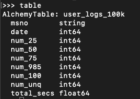
table = ibis_con.table("user_logs_100k")

The above code uses an in-memory DB with DuckDB and reads in the CSV file into a table user_logs_100k. We then create an Ibis table object from that table so we can do operations on it. Now is a good time to mention that Ibis uses lazy evaluation, so it won’t actually do any computation until we ask for a result. If we look at the table object we will be able to view the schema though.

Now we’ll want to clean up the data a little. This table has a numerical column date that is in the format YYYYMMDD (i.e. 20150101). We’ll first want to convert that into an actual date so that we can perform some operations on it, and “date” is often a reserved word, so let’s make it a different column name too:

user_logs = table.mutate(log_date = 
_.date.cast("string").to_timestamp("%Y%m%d").date()).drop("date")

The mutate command in Ibis allows us to add columns to a table. You can add multiple columns at a time, but here we just add one, log_date. This is constructed by casting our int64 date column to a string, calling the to_timestamp operator on it, then converting that to a date. We also then drop the date column. If the underscore (_) is confusing: understand that we’re using it to refer to the parent table (i.e. table). This is a little bit of syntactic sugar that can make your code easier to digest.

Now we can do some feature construction. If you look at the dataset, you might get some ideas about things you’d like to know. For example, let’s group by each user (msno) and we might want to know things like: the total number of seconds logged, the number of days the user was active, the total songs listened to, etc. Depending on the use case we may have different needs for different features, but it’ll be easy to construct these features with Ibis. Try out the following:

user_logs_agg = user_logs.aggregate(    
		by=["msno"],     
		sum_total_secs = _.total_secs.sum(),     
		avg_total_secs = _.total_secs.mean(),     
		max_total_secs = _.total_secs.max(),    
		min_total_secs = _.total_secs.min(),    
		total_days_active = _.count(),     
		first_session = _.log_date.max(),     
		most_recent_session = _.log_date.min(),    
		total_songs_listened = (_.num_25 + _.num_50 + _.num_75 + _.num_985 + _.num_100).sum(),    
		avg_num_songs_listened = (_.num_25 + _.num_50 + _.num_75 + _.num_985 + _.num_100).mean(),    
		percent_unique = (_.num_unq/(_.num_25 + _.num_50 + _.num_75 + _.num_985 + _.num_100)).mean(),
)

In the code above, we aggregate by the column msno, which is the user id column, and then we define lots of aggregated columns to create. The syntax is hopefully self-explanatory for all those shown. For example, if we want a running sum of total_secs for each user we can call _.total_secs.sum(), remembering that the underscore denotes the parent table.

Once your workflow is done, you’ll hopefully want to save the results. You can do that via the create_table expression, as shown below:

ibis_con.create_table("user_logs_agg", user_logs_agg)

This creates a table called user_logs_agg using the ibis object. If you’d rather just view the results of the query, you can do so via the execute command:

df = user_logs_agg.execute()
df.head()

Putting all the code together, here’s what our final script looks like:

import ibis 
from ibis import _

def build_features(table):
    user_logs = table.mutate(log_date = _.date.cast("string").to_timestamp("%Y%m%d").date()).drop("date")

    user_logs_agg = user_logs.aggregate(
        by=["msno"], 
        sum_total_secs = _.total_secs.sum(), 
        avg_total_secs = _.total_secs.mean(), 
        max_total_secs = _.total_secs.max(),
        min_total_secs = _.total_secs.min(),
        total_days_active = _.count(), 
        first_session = _.log_date.max(), 
        most_recent_session = _.log_date.min(),
        total_songs_listened = (_.num_25 + _.num_50 + _.num_75 + _.num_985 + _.num_100).sum(),
        avg_num_songs_listened = (_.num_25 + _.num_50 + _.num_75 + _.num_985 + _.num_100).mean(),
        percent_unique = (_.num_unq/(_.num_25 + _.num_50 + _.num_75 + _.num_985 + _.num_100)).mean(),
)
    return user_logs_agg

ibis_con = ibis.duckdb.connect() #use in-memory db
ibis_con.read_csv("./kkbox-churn-prediction-challenge/data/user_logs_100k.csv", "user_logs_100k")

table = ibis_con.table("user_logs_100k")

user_logs_featurized = build_features(table)

ibis_con.create_table("user_logs_agg", user_logs_agg)

Scaling to Spark

I promised before that we could scale our workload to Spark without changing our Ibis workflow code, so, without further ado, here’s our Spark code:

import ibis 
from ibis import _
from pyspark.sql import SparkSession 

def build_features(table):    
		user_logs = table.mutate(log_date = 
_.date.cast("string").to_timestamp("%Y%m%d").date()).drop("date")    
		user_logs_agg = user_logs.aggregate(        
				by=["msno"], 
        sum_total_secs = _.total_secs.sum(), 
        avg_total_secs = _.total_secs.mean(),
        max_total_secs = _.total_secs.max(),
        min_total_secs = _.total_secs.min(),
        total_days_active = _.count(),
        first_session = _.log_date.max(),
        most_recent_session = _.log_date.min(),
        total_songs_listened = (_.num_25 + _.num_50 + _.num_75 + _.num_985 + _.num_100).sum(),        
				avg_num_songs_listened = (_.num_25 + _.num_50 + _.num_75 + _.num_985 + _.num_100).mean(),        
				percent_unique = (_.num_unq/(_.num_25 + _.num_50 + _.num_75 + _.num_985 + _.num_100)).mean(),)    

	return user_logs_agg

session = 
SparkSession.builder.appName("kkbox-customer-churn").getOrCreate
#if you don’t use legacy mode here, you’ll need to change the timestamp formatting code 
session.conf.set("spark.sql.legacy.timeParserPolicy","LEGACY")
df = 
session.read.parquet("gs://voltrondata-demo-data/kkbox-churn/user_logs/*.parquet")
df.createOrReplaceTempView("user_logs")

()ibis_con = ibis.pyspark.connect(session)
table = ibis_con.table("user_logs")

user_logs_agg = build_features(table)
ibis_con.create_table("user_logs_agg", user_logs_agg)

The only code we change here is the code to connect to Spark. I’ve stored my user_logs files in my Google Cloud Storage account (Pro Tip: convert them to Parquet files!), but you can use any storage backend supported by Spark. Once you have a Spark DataFrame, you can register it as a view in Spark and then connect that to Ibis to start working. After that, the workflow code is exactly the same. (Pro Tip: If you get in the habit of using execute() to view your data as you iterate, be sure to add a limit() clause on your table before executing to prevent too much data from being sent back to your client.)

Closing Thoughts

Ibis can be an incredibly powerful tool for modern data teams who are looking to future-proof their data workloads. Technical debt is a real force to be reckoned with as data systems come and go, and Ibis can help companies get the most out of their data investments. Get started today by downloading Ibis and working through the documentation.

References

1 Note that dbt-python is a module that lets dbt users write Python and compiles it into Python to execute on your data warehouse. This requires that the data warehouse have a supported Python execution engine and that users are also aware of how to write in that dialect, which is quite different from what Ibis is trying to accomplish.

Photo by Ruiyang Zhang