How to Use Snowflake and Ibis for Better Analytics
By
M
Marlene MhangamiAuthor(s):
M
Marlene MhangamiPublished: March 23, 2023
6 min read
Today, data teams are growing faster than ever as businesses increasingly look to data analytics to help them make informed decisions. However, with the high number of data sources and formats, managing and processing large amounts of information can feel overwhelming. One solution to this problem is Snowflake.
Snowflake is a cloud-based data warehousing and analytics platform that offers a scalable solution for storing, processing, and analyzing data. It provides a convenient platform for data warehousing, data lakes, data engineering, and data application development. One of the key benefits of Snowflake is its cloud-native architecture, which allows it to seamlessly integrate with other cloud-based services and data sources. This makes it easy for businesses to centralize their data, while also reducing infrastructure and maintenance costs.
Why Use Ibis with Snowflake?
Snowflake is an excellent enterprise data storage solution that relies primarily on SQL for data analytics workflows. Some data engineers prefer using Python for data analysis, and SQL can be a barrier for them, particularly if they are not as experienced with writing good/performant SQL. These users might also feel more productive working from their local environment, in a Jupyter notebook for example.
Fortunately, by combining Snowflake and Ibis, engineers and data scientists get the readability of Python analytics with the scale and performance of SQL. So what is Ibis? Ibis is a pandas-like, Python library that provides a lightweight, universal interface for data wrangling. It helps Python users explore and transform data of any size, stored anywhere. With Ibis, data analysts and engineers can write Python code that generates SQL queries and pipelines. For Snowflake users, Ibis generates the SQL code necessary to query data stored in their Snowflake database and the results are returned natively in their local Python environment. Ibis also allows users to access the generated SQL code by using the show_sql command
Creating A Pricing Summary Report
As an example of what using Ibis and Snowflake together looks like, we’ll prepare a short pricing summary report. We’ll work with Ibis in a Jupyter notebook in our local IDE to connect to Snowflake and grab a table that has information about a business’s shipping, sales, and returns data. We’ll generate a pricing summary report that helps us understand how the business performed in a certain time interval. Let’s start by installing the Ibis-Snowflake backend using the code below.
install ibis-snowflake backend
python
!pip install 'ibis-framework[snowflake]'Next, we’ll import all the necessary dependencies to get going and connect to the Snowflake database using ibis.connect.
The ibis.connect function takes in a URL that looks like this"snowflake://user:pass@account/database/schema".
The parts of this url are made up of:
- Snowflake username (listed under your profile tab)
- Snowflake password (hopefully you know this ;))
- Snowflake account:
- You’ll find this under the Admin→Accounts tab in the menu. Clicking on the link next to the letters under the ‘Account’ section on this page will give you a URL that looks something like this
https://abcdefg-rr01234.snowflakecomputing.com. Your account consists of all the letters and numbers beforesnowflakecomputing.comso in this case, it would beabcdefg-rr01234
- You’ll find this under the Admin→Accounts tab in the menu. Clicking on the link next to the letters under the ‘Account’ section on this page will give you a URL that looks something like this
- Database name
- Schema name
Once you have your URL, you can plug it in and run the following code to connect to the Snowflake database. This gives you access to all the tables available in your chosen database.
import dependencies and connect to the Snowflake backend
python
import ibis
from ibis import _
ibis.options.interactive = True

con = ibis.connect(
    "snowflake://user:pass@account/database/schema"
)
For this example, we’ll use the Snowflake-provided ‘snowflake_sample_data’ database. From this database, we’ll use the lineitem table. We can connect to the table by running this line of code.
connect to the lineitem table
python
lineitem = con.tables.lineitemWe’ll now use Ibis to generate a short report that shows the amount of business that was billed, shipped, and returned as of a given date. Our query will list the totals for extended price, discounted extended price, price with tax, average quantity, average price, and average discount. These aggregates are grouped by RETURNFLAG and LINESTATUS and listed in ascending order of the same. A count of the number of line items in each group is included.
create the report
python
report = lineitem.aggregate(
    by=['L_RETURNFLAG','L_LINESTATUS'],
    sum_qty = _.L_QUANTITY .sum(),
    sum_base_price = _.L_EXTENDEDPRICE.sum(),
    sum_disc_price = (_.L_EXTENDEDPRICE * (1-_.L_DISCOUNT)).sum(),
    sum_charge = (_.L_EXTENDEDPRICE * (1-_.L_DISCOUNT) * (1+_.L_TAX)).sum(),
    avg_qty = _.L_QUANTITY .mean(),
    avg_price = _.L_EXTENDEDPRICE.mean(),
    avg_disc = _.L_DISCOUNT.mean(),
    count_order = _.count()
).filter(lineitem.L_SHIPDATE <'1998-12-01').order_by(['L_RETURNFLAG','L_LINESTATUS'])

report
python
┏━━━━━━━━━━━━━━┳━━━━━━━━━━━━━━┳━━━━━━━━━━━━━━━━┳━━━━━━━━━━━━━━━━━┳━━━━━━━━━━━━━━━━━━━┳━━━━━━━━━━━━━━━━━━━━━┳━━━━━━━━━━━━━━━━┳━━━━━━━━━━━━━━━━┳━━━━━━━━━━━━━━━━┳━━━━━━━━━━━━━┓
┃ L_RETURNFLAG ┃ L_LINESTATUS ┃ sum_qty ┃ sum_base_price ┃ sum_disc_price ┃ sum_charge ┃ avg_qty ┃ avg_price ┃ avg_disc ┃ count_order ┃
┡━━━━━━━━━━━━━━╇━━━━━━━━━━━━━━╇━━━━━━━━━━━━━━━━╇━━━━━━━━━━━━━━━━━╇━━━━━━━━━━━━━━━━━━━╇━━━━━━━━━━━━━━━━━━━━━╇━━━━━━━━━━━━━━━━╇━━━━━━━━━━━━━━━━╇━━━━━━━━━━━━━━━━╇━━━━━━━━━━━━━┩
│ !string │ !string │ decimal(38, 2) │ decimal(38, 2) │ decimal(38, 4) │ decimal(38, 6) │ decimal(12, 2) │ decimal(12, 2) │ decimal(12, 2) │ int64 │
├──────────────┼──────────────┼────────────────┼─────────────────┼───────────────────┼─────────────────────┼────────────────┼────────────────┼────────────────┼─────────────┤
│ A │ F │ 37734107.00 │ 56586554400.73 │ 53758257134.8700 │ 55909065222.827690 │ 25.52 │ 38273.13 │ 0.05 │ 1478493 │
│ N │ F │ 991417.00 │ 1487504710.38 │ 1413082168.0541 │ 1469649223.194375 │ 25.52 │ 38284.47 │ 0.05 │ 38854 │
│ N │ O │ 76633518.00 │ 114935210409.19 │ 109189591897.4720 │ 113561024263.013779 │ 25.50 │ 38248.02 │ 0.05 │ 3004998 │
│ R │ F │ 37719753.00 │ 56568041380.90 │ 53741292684.6040 │ 55889619119.831932 │ 25.51 │ 38250.85 │ 0.05 │ 1478870 │
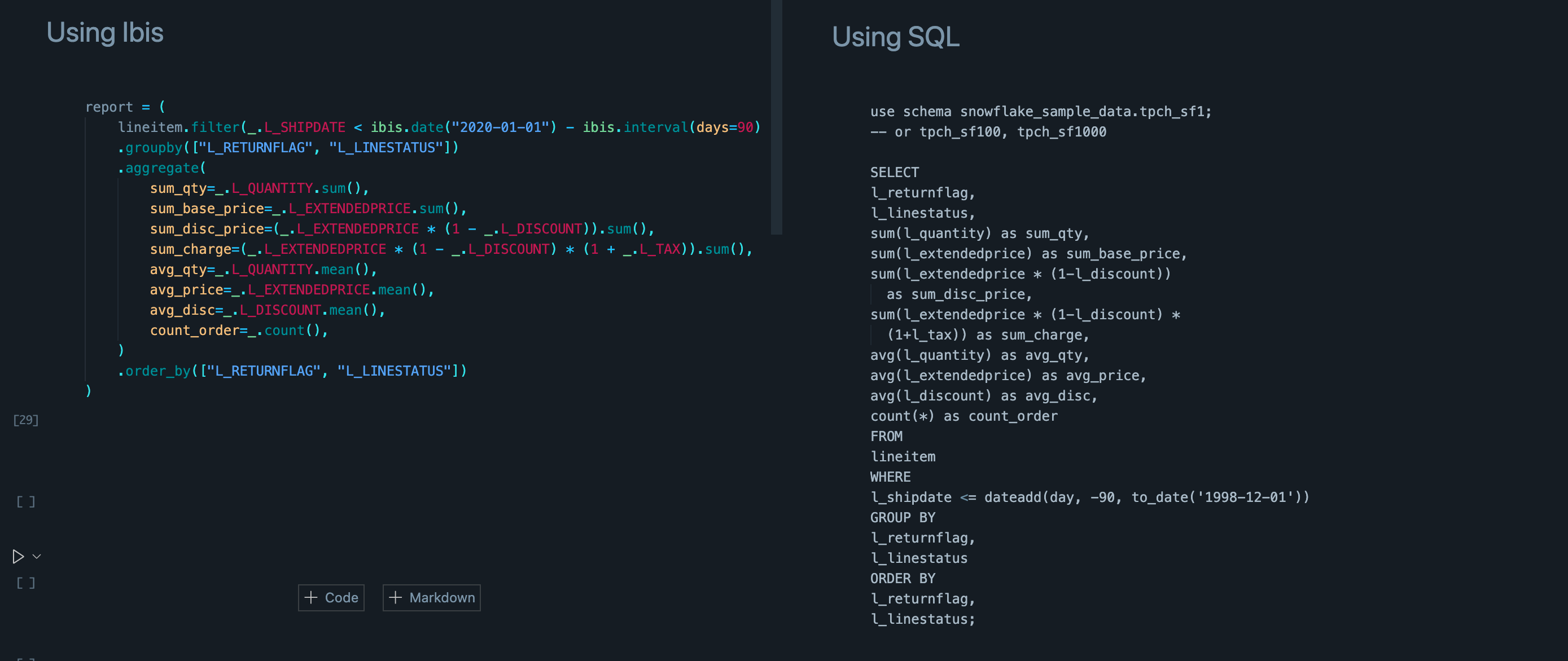
└──────────────┴──────────────┴────────────────┴─────────────────┴───────────────────┴─────────────────────┴────────────────┴────────────────┴────────────────┴─────────────┘Ibis uses Rich under the hood so tables are presented in a clear way. For more perspective, here’s a side-by-side comparison of the SQL query needed to generate the same results and our Ibis query. For Python users, Ibis should feel more intuitive and lightweight. This entire workflow was also completed in a Jupyter notebook in a local IDE.
Conclusion
In summary, Snowflake is a powerful data warehousing and analytics platform, and using it with Ibis provides software engineers and data scientists more flexibility. By using Ibis, data teams can unlock the full potential of their analytics workflows, while still benefiting from the scalability, reliability, and security of Snowflake’s cloud-based infrastructure.
If you’re interested in building a data analytics system that uses the power of Snowflake and Ibis, don’t hesitate to reach out to our team at hello@voltrondata.com. We specialize in helping data teams leverage these technologies to gain valuable insights from their data and make informed decisions.
Photo by Kelly
Previous Article

Keep up with us