Adding A New Ibis-cuDF Backend With Zero Code Changes
By
M
Marlene MhangamiandN
Nick BeckerAuthor(s):
M
Marlene MhangamiN
Nick BeckerPublished: December 15, 2023
6 min read
TL;DR: cudf.pandas (pandas accelerator mode) is a new extension from the RAPIDS cuDF team that leverages the power of GPUs to improve pandas performance. By executing on the GPU where possible and on the CPU otherwise, this new mode provides major speedups with zero code changes to existing pandas workflows. Ibis was able to add a new cuDF backend by using its existing pandas backend with the cudf.pandas extension.
The RAPIDS team at NVIDIA just announced that v23.10 of cuDF includes a pandas accelerator mode (cudf.pandas), a feature that offers a unified CPU/GPU experience. This new mode brings GPU-acceleration to pandas workflows with zero code changes. With cudf.pandas, operations execute on the GPU where possible and on the CPU (using pandas) otherwise, synchronizing under the hood as needed.
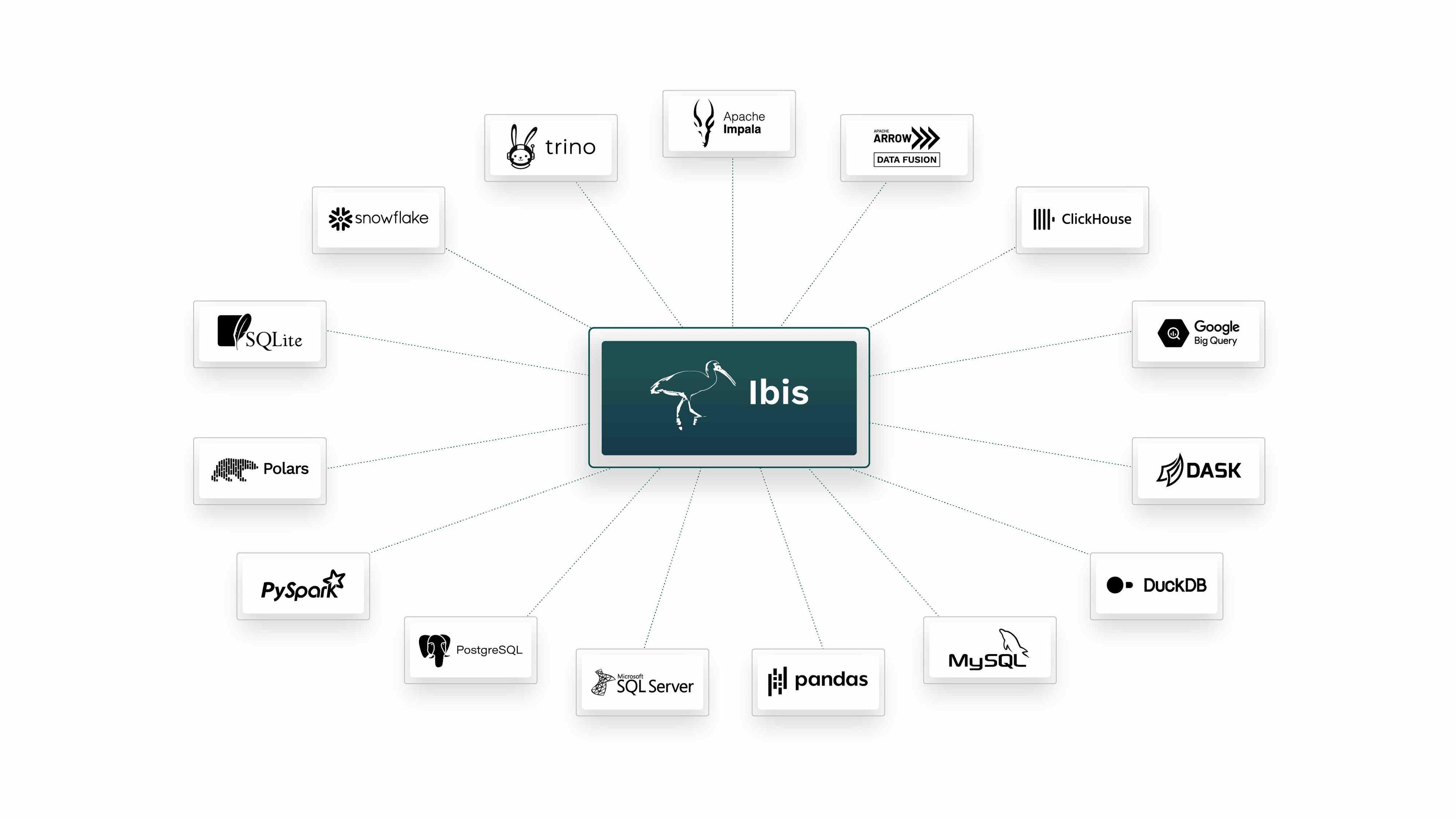
The new pandas accelerator mode is exciting and useful for a number of different reasons. One use case that stands out for me is with Ibis. If you’ve been following the Voltron Data blog you’ll know that Ibis is one of the flagship open source libraries that we support. Ibis is “the portable Python dataframe library” that gives you the flexibility of a pandas-like API with the ability to target one of many SQL and DataFrame engines as a backend for high performance and portability. Currently, Ibis supports 17+ backends including MySQL, SnowflakeDB, DuckDB, Trino, Google BigQuery and pandas.
For SQL backends, under the hood Ibis takes your Python code, translates it to the specific flavor of SQL, optimizes it and then returns the results of the query. Ibis also uses lazy execution (executing a query and pulling in data only when necessary) to ensure your workflow is as efficient as possible in terms of both memory and speed. Building composable data systems with libraries like Ibis makes it less challenging and less expensive to work with multiple database engines. For example if you’re using SQL on a cloud platform that encourages lock-in, you don’t need to change your code when switching between cloud platforms or from cloud to on-prem systems. Check out an example blog I wrote using Ibis with BigQuery here.
Unlike the SQL backends, there are fewer DataFrame backends in Ibis and implementing new ones is non-trivial. Ibis currently has a pandas backend but the problems with performance that often plague pandas users still persist, making it a less than ideal choice for most.
Using cudf.pandas, we were able to add a new cuDF backend to Ibis with zero code changes, giving the pandas backend a huge speedup!
Using Ibis-cuDF
All Ibis users can test out this new backend today by installing the latest version of cuDF and turning on pandas accelerator mode. Since Ibis is a universal DataFrame front-end, not only can you switch between CPU-based backends without changing your workflow — you can now flexibly switch between CPU and GPU systems as needed to maximize your workflows performance.
To install cuDF run this in the command line to install with PIP or visit this page for instructions for conda.
bash
# If you’re using CUDA 11, install cudf-cu11 instead

pip install \
    --extra-index-url=https://pypi.nvidia.com \
    cudf-cu12
Next, let’s switch to a Jupyter Notebook and look at some performance comparisons. In the examples below, we’ll process a synthetic 100 million row dataset on an Intel Xeon Platinum 8480CL CPU and an NVIDIA H100 GPU.
We’ll start off by importing pandas and ibis and explicitly setting the ibis backend to pandas. It’s important to note that we haven’t yet activated cudf.pandas, so this is how long it takes to do some operations with ibis-pandas.
python
import pandas as pd
import ibis
import numpy as np

ibis.options.interactive = True
ibis.set_backend("pandas")
Let’s create a pandas dataframe and turn it into an ibis-pandas table by feeding it to the ibis.memtable function as shown below.
python
N = 100000000
K = 5

rng = np.random.default_rng(12)

df = pd.DataFrame(
    rng.normal(10, 5, (N, K)),
    columns=[f"c{x}" for x in np.arange(K)]
)

df["key"] = rng.choice(np.arange(10), N)
df["s"] = rng.choice(["Hello", "World", "It's", "Me", "Again"], N)

t = ibis.memtable(df, name="t")
Table t is now an ibis-pandas table. Below we’re running two group-bys on the table and getting the time they take to run.
python
%%time

res = t.group_by("key").agg(
  total_cost=t.c0.sum(),
     avg_cost=t.c0.mean()
).order_by("key")
print(res)

┏━━━━━━━┳━━━━━━━━━━━━━━┳━━━━━━━━━━━┓
┃ key   ┃ total_cost   ┃ avg_cost  ┃
┡━━━━━━━╇━━━━━━━━━━━━━━╇━━━━━━━━━━━┩
│ int64 │ float64      │ float64   │
├───────┼──────────────┼───────────┤
│     0 │ 9.996313e+07 │  9.996527 │
│     1 │ 1.000396e+08 │ 10.000438 │
│     2 │ 9.997690e+07 │ 10.001319 │
│     3 │ 1.000144e+08 │  9.999324 │
│     4 │ 1.000225e+08 │  9.999703 │
│     5 │ 1.000276e+08 │ 10.000437 │
│     6 │ 9.994562e+07 │ 10.001741 │
│     7 │ 9.999089e+07 │  9.997739 │
│     8 │ 9.998734e+07 │  9.998644 │
│     9 │ 1.000069e+08 │ 10.001611 │
└───────┴──────────────┴───────────┘
CPU times: user 1.69 s, sys: 276 ms, total: 1.97 s
Wall time: 1.97 s
python
%%time

res = t.group_by("key").order_by("c2").mutate(lagged_diff=t.c4 - t.c4.lag()).limit(10)
print(res)

┏━━━━━━━━━━━┳━━━━━━━━━━━┳━━━━━━━━━━━┳━━━━━━━━━━━┳━━━━━━━━━━━┳━━━━━━━┳━━━━━━━━┳━━━━━━━━━━━━━┓
┃ c0        ┃ c1        ┃ c2        ┃ c3        ┃ c4        ┃ key   ┃ s      ┃ lagged_diff ┃
┡━━━━━━━━━━━╇━━━━━━━━━━━╇━━━━━━━━━━━╇━━━━━━━━━━━╇━━━━━━━━━━━╇━━━━━━━╇━━━━━━━━╇━━━━━━━━━━━━━┩
│ float64   │ float64   │ float64   │ float64   │ float64   │ int64 │ string │ float64     │
├───────────┼───────────┼───────────┼───────────┼───────────┼───────┼────────┼─────────────┤
│  9.965866 │ 15.230716 │ 13.707942 │ 13.619783 │ 18.093881 │     9 │ Again  │   3.268698 │
│  3.972209 │  6.865223 │  3.396684 │  9.461237 │ 14.993818 │     6 │ Hello  │   3.754521 │
│  9.890261 │ 12.479400 │  0.446157 │ 10.735321 │  5.465284 │     2 │ Me     │ -13.901625 │
│ 18.876947 │ 14.434245 │ 14.746747 │  9.710725 │ 13.064311 │     1 │ Hello  │   3.582080 │
│ 13.289451 │  8.277987 │  7.513140 │  9.426136 │  6.972740 │     5 │ Hello  │  -7.940455 │
│  7.028303 │  8.583123 │  6.357911 │ 13.831639 │  2.019568 │     7 │ World  │ -10.140622 │
│ 14.117811 │  6.872168 │  7.270300 │  3.245764 │  9.278789 │     1 │ Me     │  -7.232555 │
│  8.761692 │ 10.957279 │  7.331129 │ 10.468781 │ 19.098459 │     9 │ World  │   7.142314 │
│ 12.044998 │  7.131550 │ 14.765548 │  9.355994 │ 12.969372 │     0 │ World  │   3.487767 │
│ 13.063737 │  8.044671 │  0.348563 │  8.261732 │ 12.757277 │     8 │ Me     │   6.416780 │
└───────────┴───────────┴───────────┴───────────┴───────────┴───────┴────────┴────────────┘
CPU times: user 3min 29s, sys: 23.7 s, total: 3min 53s
Wall time: 3min 53s
With 100 million records, the basic group_by aggregation takes a couple of seconds with the pandas backend. But the more complex group_by mutate operation to calculate lagged differences is very slow, taking nearly four minutes. Things would only get worse as data sizes grow.
Let’s turn on cudf.pandas to see if we can speed things up. To do this, I’ll simply load the Jupyter Notebook extension before I import pandas.
python
%load_ext cudf.pandas

import pandas as pd
import ibis
import numpy as np

ibis.options.interactive = True
ibis.set_backend("pandas")
And that’s it. I can run the exact same code I had in the cells above and use cuDF as a backend for Ibis.
python
%%time

res = t.group_by("key").agg(
  total_cost=t.c0.sum(),
     avg_cost=t.c0.mean()
).order_by("key")
print(res)

┏━━━━━━━┳━━━━━━━━━━━━━━┳━━━━━━━━━━━┓
┃ key   ┃ total_cost   ┃ avg_cost  ┃
┡━━━━━━━╇━━━━━━━━━━━━━━╇━━━━━━━━━━━┩
│ int64 │ float64      │ float64   │
├───────┼──────────────┼───────────┤
│     0 │ 9.996313e+07 │  9.996527 │
│     1 │ 1.000396e+08 │ 10.000438 │
│     2 │ 9.997690e+07 │ 10.001319 │
│     3 │ 1.000144e+08 │  9.999324 │
│     4 │ 1.000225e+08 │  9.999703 │
│     5 │ 1.000276e+08 │ 10.000437 │
│     6 │ 9.994562e+07 │ 10.001741 │
│     7 │ 9.999089e+07 │  9.997739 │
│     8 │ 9.998734e+07 │  9.998644 │
│     9 │ 1.000069e+08 │ 10.001611 │
└───────┴──────────────┴───────────┘
CPU times: user 212 ms, sys: 67.8 ms, total: 280 ms
Wall time: 287 ms
python
%%time

res = t.group_by("key").order_by("c2").mutate(lagged_diff=t.c4 - t.c4.lag()).limit(10)
print(res)

┏━━━━━━━━━━━┳━━━━━━━━━━━┳━━━━━━━━━━━┳━━━━━━━━━━━┳━━━━━━━━━━━┳━━━━━━━┳━━━━━━━━┳━━━━━━━━━━━━━┓
┃ c0        ┃ c1        ┃ c2        ┃ c3        ┃ c4        ┃ key   ┃ s      ┃ lagged_diff ┃
┡━━━━━━━━━━━╇━━━━━━━━━━━╇━━━━━━━━━━━╇━━━━━━━━━━━╇━━━━━━━━━━━╇━━━━━━━╇━━━━━━━━╇━━━━━━━━━━━━━┩
│ float64   │ float64   │ float64   │ float64   │ float64   │ int64 │ string │ float64     │
├───────────┼───────────┼───────────┼───────────┼───────────┼───────┼────────┼─────────────┤
│  9.965866 │ 15.230716 │ 13.707942 │ 13.619783 │ 18.093881 │     9 │ Again  │   3.268698 │
│  3.972209 │  6.865223 │  3.396684 │  9.461237 │ 14.993818 │     6 │ Hello  │   3.754521 │
│  9.890261 │ 12.479400 │  0.446157 │ 10.735321 │  5.465284 │     2 │ Me     │ -13.901625 │
│ 18.876947 │ 14.434245 │ 14.746747 │  9.710725 │ 13.064311 │     1 │ Hello  │   3.582080 │
│ 13.289451 │  8.277987 │  7.513140 │  9.426136 │  6.972740 │     5 │ Hello  │  -7.940455 │
│  7.028303 │  8.583123 │  6.357911 │ 13.831639 │  2.019568 │     7 │ World  │ -10.140622 │
│ 14.117811 │  6.872168 │  7.270300 │  3.245764 │  9.278789 │     1 │ Me     │  -7.232555 │
│  8.761692 │ 10.957279 │  7.331129 │ 10.468781 │ 19.098459 │     9 │ World  │   7.142314 │
│ 12.044998 │  7.131550 │ 14.765548 │  9.355994 │ 12.969372 │     0 │ World  │   3.487767 │
│ 13.063737 │  8.044671 │  0.348563 │  8.261732 │ 12.757277 │     8 │ Me     │   6.416780 │
└───────────┴───────────┴───────────┴───────────┴───────────┴───────┴────────┴────────────┘
CPU times: user 456 ms, sys: 112 ms, total: 567 ms
Wall time: 585 ms
As you can see, in both cases switching to cuDF significantly improved performance. In particular, calculating per-group lagged differences was much faster — from four minutes to 0.5 seconds!
This makes sense. The lagged differences operation is much more complex than the basic group_by sum and mean.
Conclusion
Using the cuDF backend with ibis isn’t always the right choice. For many workloads, high-performance CPU-based engines like DuckDB or your favorite cloud engine will make the most sense. But for performance critical, complex workflows, cuDF’s pandas accelerator mode can be a great choice.
From our initial testing, it’s particularly well suited to Ibis workflows using group_by in conjunction with mutate on 5-25 GBs of data. If that sounds like some of your workflows, give it a try!
Previous Article

Keep up with us