Passing Arrow Data Between R and Python with Reticulate
By
D
Danielle NavarroAuthor(s):
D
Danielle NavarroPublished: September 27, 2022
15 min read
This article originally appeared on Danielle Navarro’s blog.
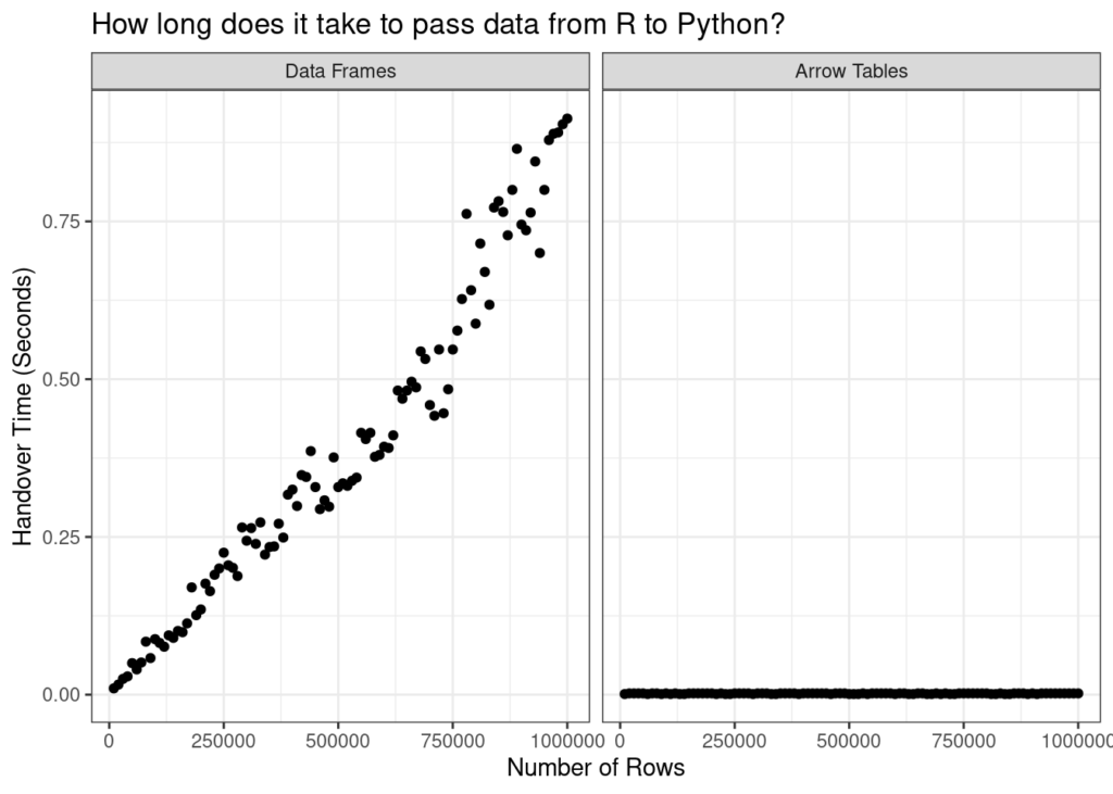
An ad-hoc comparison of effort to pass datasets of varying sizes from R to Python without Arrow (left) and with Arrow (right).
Data Interchange in a Polyglot World
As data science moves toward a “polyglot” ethos that emphasizes the importance of multi-language tools, it’s becoming more common to pass data sets back and forth between different languages. With that in mind, this post is a primer on how to efficiently pass control of an Apache Arrow data set between R and Python without making any wasteful copies of the data.
Reticulate seems so smooth and seamless without Arrow, you may be wondering if it’s even necessary to use Arrow. The example in the first section below only looks smooth and seamless because the data set is small. As I’ll show later in the post, cracks in the facade start to appear when you have to pass large data sets across languages. This happens for the very simple reason that a Pandas DataFrame is a different thing to an R data frame. It’s not possible for the two languages to share a single copy of the same data object because they don’t agree on what constitutes “a data object.” The only way we can do the handover is to make a copy of the data set and convert it to a format more suitable to the destination language. When the data set is small, this is not a problem. But as your data set grows, this becomes ever more burdensome. These copy-and-convert operations are not cheap.
Wouldn’t it be nice if R and Python could both agree to represent the data as, oh let’s say…. an Arrow Table? On the R side we could interact with it using the arrow R package, and on the Python side we could interact with it using the pyarrow module. But regardless of which language we’re using, the thing in memory would be exactly the same… handing over the data set from one language to the other would no longer require any copying. A little metadata would change hands, and that’s all.
The idea to write this post emerged from a recent discussion on Twitter started by Cass Wilkinson Saldaña about passing control of a data set from R to Python, and a comment in that discussion by Jon Keane mentioning that with the assistance of Apache Arrow this handover can be made very smooth, and incredibly efficient too. In this post, I’ll unpack this a little and explain how the magic works. As usual I’ll start by loading some packages:
r
library(tidyverse)
library(tictoc)
The Reticulate Trick
The “trick” is simple: if your data are stored as an Arrow Table, and you use the reticulate package to pass it from R to Python (or vice versa), only the metadata changes hands. Because an Arrow Table has the same structure in-memory when accessed from Python as it does in R, the data set itself does not need to be touched at all. The only thing that needs to happen is the language on the receiving end needs to be told where the data are stored. Or, to put it another way, we just pass a pointer across. This all happens invisibly, so if you know how to use reticulate[1], you already know almost everything you need to know and can skip straight to the section on passing Arrow objects. If you’re like Danielle-From-Last-Month and have absolutely no idea how reticulate works, read on…
Managing the Python environment from R
If reticulate is not already on your system, you can install it from CRAN with install.packages("reticulate"). Once installed, you can load it in the usual fashion:
r
library(reticulate)What happens next depends a little on your Python setup. If you don’t have a preferred Python configuration on your machine already and would like to let reticulate manage everything for you, then you can do something like this:
r
install_python()
install_miniconda()
This will set you up with a default Python build, managed by a copy of Miniconda that it installs in an OS-specific location that you can discover by calling miniconda_path().
The previous approach is a perfectly sensible way to use reticulate, but in the end I went down a slightly different path. I already had Python and Miniconda configured on my local machine, and I didn’t want reticulate to install new versions that might make a mess of things[2]. If you’re in a similar position, you probably want to use your existing Python set up and ensure that reticulate knows where to find everything. If that’s the case, what you want to do is edit your .Renviron file[3] and set the RETICULATE_MINICONDA_PATH variable. Add a line like this one:
renviron
RETICULATE_MINICONDA_PATH=/home/danielle/miniconda3/(where you should specify the path to your Miniconda installation, not mine.)
Regardless of which method you’ve followed, you can use conda_list() to display a summary of all your Python environments.[4] In truth, I haven’t used Python much on this machine, so my list of environments is short:
r
conda_list()
          name                                                 python
1         base                   /home/danielle/miniconda3/bin/python
2 continuation /home/danielle/miniconda3/envs/continuation/bin/python
3 r-reticulate /home/danielle/miniconda3/envs/r-reticulate/bin/python
4       tf-art       /home/danielle/miniconda3/envs/tf-art/bin/python
For the purposes of this post I’ll create a new environment that I will call “reptilia”, in line with the data that I’ll be analyzing later. To keep things neat I’ll install[5] the pandas and pyarrow packages that this post will be using at the same time:
r
conda_create(
  envname = "reptilia",
  packages = c("pandas", "pyarrow")
)
Having done this, I can call conda_list() again, and when R lists my conda environments I see that the reptilia environment now exists:
r
conda_list()
          name                                                 python
1         base                   /home/danielle/miniconda3/bin/python
2 continuation /home/danielle/miniconda3/envs/continuation/bin/python
3 r-reticulate /home/danielle/miniconda3/envs/r-reticulate/bin/python
4     reptilia     /home/danielle/miniconda3/envs/reptilia/bin/python
5       tf-art       /home/danielle/miniconda3/envs/tf-art/bin/python
To ensure that reticulate uses the reptilia environment throughout,[6] I call the use_miniconda() function and specify the environment name:
r
use_miniconda("reptilia")Our set up is now complete!
Using reticulate to call Python from R
Now that my environment is set up I’m ready to use Python. When calling Python code from within R, some code translation is necessary due to the differences in syntax across languages. As a simple example, let’s say I have my regular Python session open and I want to check my Python version and executable. To do this I’d import the sys library:
python
import sys
print(sys.version)
print(sys.executable)

-------
3.8.13 | packaged by conda-forge | \(default, Mar 25 2022, 06:15:10)
[GCC 10.3.0]
/home/danielle/miniconda3/envs/reptilia/bin/python
To execute these commands from R, the code needs some minor changes. The import() function replaces the import keyword, and $ replaces . as the accessor:
r
sys <- import("sys")
sys$version
sys$executable

-------
[1] "3.8.13 | packaged by conda-forge | \(default, Mar 25 2022, 06:15:10) \n[GCC 10.3.0]"
[1] "/home/danielle/miniconda3/envs/reptilia/bin/python"
The code looks more R-like, but Python is doing the work.[7]
Copying data frames between languages
Okay, now that we understand the basics of reticulate, it’s time to tackle the problem of transferring data sets between R and Python. For now, let’s leave Arrow out of this. All we’re going to do is take an ordinary R data frame and transfer it to Python.
First, let’s load some data into R. The data are taken from The Reptile Database (accessed August 31 2022), an open and freely available catalog of reptile species and their scientific classifications.[8]
r
taxa <- read_csv2("taxa.csv")
taxa
# A tibble: 14,930 × 10
taxon_id family subfa…¹ genus subge…² speci…³ autho…⁴ infra…⁵ infra…⁶ infra…⁷
1 Ablepha… Scinc… Eugong… Able… NA alaicus ELPATJ…
2 Ablepha… Scinc… Eugong… Able… NA alaicus ELPATJ… subsp. alaicus ELPATJ…
3 Ablepha… Scinc… Eugong… Able… NA alaicus ELPATJ… subsp. kucenk… NIKOLS…
4 Ablepha… Scinc… Eugong… Able… NA alaicus ELPATJ… subsp. yakovl… (EREMC…
5 Ablepha… Scinc… Eugong… Able… NA anatol… SCHMID…
6 Ablepha… Scinc… Eugong… Able… NA bivitt… (MENET…
7 Ablepha… Scinc… Eugong… Able… NA budaki GÖCMEN…
8 Ablepha… Scinc… Eugong… Able… NA cherno… DAREVS…
9 Ablepha… Scinc… Eugong… Able… NA cherno… DAREVS… subsp. cherno… DAREVS…
10 Ablepha… Scinc… Eugong… Able… NA cherno… DAREVS… subsp. eiselti SCHMID…
#… with 14,920 more rows, and abbreviated variable names ¹subfamily,
# ²subgenus, ³specific_epithet, ⁴authority, ⁵infraspecific_marker,
# ⁶infraspecific_epithet, ⁷infraspecific_authorityCurrently this object is stored in-memory as an R data frame and we want to move it to Python. However, because Python data structures are different from R data structures, what this actually requires us to do is make a copy of the whole data set inside Python, using a Python-native data structure (in this case a Pandas DataFrame). Thankfully, reticulate does this seamlessly with the r_to_py() function:
r
py_taxa <- r_to_py(taxa)
py_taxa
                            taxon_id  ...    infraspecific_authority
0                 Ablepharus_alaicus  ...                         NA
1         Ablepharus_alaicus_alaicus  ...          ELPATJEVSKY, 1901
2        Ablepharus_alaicus_kucenkoi  ...             NIKOLSKY, 1902
3      Ablepharus_alaicus_yakovlevae  ...         (EREMCHENKO, 1983)
4              Ablepharus_anatolicus  ...                         NA
...                              ...  ...                        ...
14925           Zygaspis_quadrifrons  ...                         NA
14926               Zygaspis_vandami  ...                         NA
14927     Zygaspis_vandami_arenicola  ...  BROADLEY & BROADLEY, 1997
14928       Zygaspis_vandami_vandami  ...         (FITZSIMONS, 1930)
14929              Zygaspis_violacea  ...                         NA

[14930 rows x 10 columns]
Within the Python session, an object called r has been created: the Pandas DataFrame object is stored as r.py_taxa, and we can manipulate it using Python code in whatever fashion we normally might.
It helps to see a concrete example. To keep things simple, let’s pop over to our Python session and give ourselves a simple data wrangling task. Our goal is to count the number of entries in the data set for each reptilian family using Pandas syntax:
r
counts = r. \
  py_taxa[["family", "taxon_id"]]. \
  groupby("family"). \
  agg(len)

counts
                 taxon_id
family
Acrochordidae           3
Agamidae              677
Alligatoridae          16
Alopoglossidae         32
Amphisbaenidae        206
...                   ...
Xenodermidae           30
Xenopeltidae            2
Xenophidiidae           2
Xenosauridae           15
Xenotyphlopidae         1

[93 rows x 1 columns]
I could have done this in R using dplyr functions, but that’s not the point of the post. What matters for our purposes is that counts is a Pandas DataFrame that now exists in the Python session, which we would like to pull back into our R session.
This turns out to be easier than I was expecting. The reticulate package exposes an object named py to the user, and any objects I created in my Python session can be accessed that way:
r
py$counts
                   taxon_id
Acrochordidae             3
Agamidae                677
Alligatoridae            16
Alopoglossidae           32
Amphisbaenidae          206
Anguidae                113
Aniliidae                 3
Anomalepididae           23
Anomochilidae             3
...
What’s especially neat is that the data structure has been automatically translated for us: the counts object in Python is a Pandas DataFrame, but when accessed from R it is automatically translated into a native R data structure: py$counts is a regular data frame: [R code]
class(py$counts)
[1] "data.frame"
Data Interchange with Arrow in the Polyglot World
As mentioned in the beginning, this seems inexpensive now, but if our dataset grows we’re going to need Arrow to facilitate zero-copy data objects that can be shared between a Pandas Data Frame and an R Data Frame. Otherwise our memory is going to be taxed at 2 times the rate of the dataset growth as we’re having to duplicate the data to translate between Python and R.
Setting up Arrow
I’m not going to talk much about setting up arrow for R in this post, because I’ve written about it before! In addition to the installation instructions on the Arrow documentation there’s a getting started with Arrow post on my personal blog. But in any case, it’s usually pretty straightforward: you can install the arrow R package from CRAN in the usual way using install.packages(“arrow”) and then load it in the usual fashion:
r
library(arrow)On the Python side, I’ve already installed pyarrow earlier when setting up the “reptilia” environment. But had I not done so, I could redress this now using conda_install() with a command such as this:
r
conda_install(
  packages = "pyarrow",
  envname = "reptilia"
)
From there we’re good to go. On the R side, let’s start by reading the reptiles data directly from file into an Arrow Table:
r
taxa_arrow <- read_delim_arrow(
  file = "taxa.csv",
  delim = ";",
  as_data_frame = FALSE
)
taxa_arrow
Table
14930 rows x 10 columns
$taxon_id
$family
$subfamily
$genus
$subgenus
$specific_epithet
$authority
$infraspecific_marker
$infraspecific_epithet
$infraspecific_authority
Next let’s import pyarrow on the Python side and check the version:[9]
python
import pyarrow as pa
pa.__version__
'8.0.0'
Everything looks good here too!
Handover to Python
After all that set up, it’s almost comically easy to do the transfer itself. It’s literally the same as last time: we call r_to_py(). The taxa_arrow variable refers to an Arrow Table on the R side, so now all I have to do is use r_to_py() to create py_taxa_arrow, a variable that refers to the same Arrow Table from the Python side:
r
py_taxa_arrow <- r_to_py(taxa_arrow)
Since we’re in Python now, let’s just switch languages and take a peek, shall we? Just like last time, objects created by reticulate are accessible on the Python side via the r object, so we access this object in Python with r.py_taxa_arrow:
python
r.py_taxa_arrow
pyarrow.Table
taxon_id: string
family: string
subfamily: string
genus: string
subgenus: null
specific_epithet: string
authority: string
infraspecific_marker: string
infraspecific_epithet: string
infraspecific_authority: string
----
taxon_id: [["Ablepharus_alaicus","Ablepharus_alaicus_alaicus","Ablepharus_alaicus_kucenkoi","Ablepharus_alaicus_yakovlevae","Ablepharus_anatolicus",...,"Plestiodon_egregius_onocrepis","Plestiodon_egregius_similis","Plestiodon_elegans","Plestiodon_fasciatus","Plestiodon_finitimus"],["Plestiodon_gilberti","Plestiodon_gilberti_cancellosus","Plestiodon_gilberti_gilberti","Plestiodon_gilberti_placerensis","Plestiodon_gilberti_rubricaudatus",...,"Zygaspis_quadrifrons","Zygaspis_vandami","Zygaspis_vandami_arenicola","Zygaspis_vandami_vandami","Zygaspis_violacea"]]
family: [["Scincidae","Scincidae","Scincidae","Scincidae","Scincidae",...,"Scincidae","Scincidae","Scincidae","Scincidae","Scincidae"],["Scincidae","Scincidae","Scincidae","Scincidae","Scincidae",...,"Amphisbaenidae","Amphisbaenidae","Amphisbaenidae","Amphisbaenidae","Amphisbaenidae"]]
subfamily: [["Eugongylinae","Eugongylinae","Eugongylinae","Eugongylinae","Eugongylinae",...,"Scincinae","Scincinae","Scincinae","Scincinae","Scincinae"],["Scincinae","Scincinae","Scincinae","Scincinae","Scincinae",...,null,null,null,null,null]]
genus: [["Ablepharus","Ablepharus","Ablepharus","Ablepharus","Ablepharus",...,"Plestiodon","Plestiodon","Plestiodon","Plestiodon","Plestiodon"],["Plestiodon","Plestiodon","Plestiodon","Plestiodon","Plestiodon",...,"Zygaspis","Zygaspis","Zygaspis","Zygaspis","Zygaspis"]]
subgenus: [11142 nulls,3788 nulls]
specific_epithet: [["alaicus","alaicus","alaicus","alaicus","anatolicus",...,"egregius","egregius","elegans","fasciatus","finitimus"],["gilberti","gilberti","gilberti","gilberti","gilberti",...,"quadrifrons","vandami","vandami","vandami","violacea"]]
authority: [["ELPATJEVSKY, 1901","ELPATJEVSKY, 1901","ELPATJEVSKY, 1901","ELPATJEVSKY, 1901","SCHMIDTLER, 1997",...,"BAIRD, 1858","BAIRD, 1858","(BOULENGER, 1887)","(LINNAEUS, 1758)","OKAMOTO & HIKIDA, 2012"],["(VAN DENBURGH, 1896)","(VAN DENBURGH, 1896)","(VAN DENBURGH, 1896)","(VAN DENBURGH, 1896)","(VAN DENBURGH, 1896)",...,"(PETERS, 1862)","(FITZSIMONS, 1930)","(FITZSIMONS, 1930)","(FITZSIMONS, 1930)","(PETERS, 1854)"]]
infraspecific_marker: [[null,"subsp.","subsp.","subsp.",null,...,"subsp.","subsp.",null,null,null],[null,"subsp.","subsp.","subsp.","subsp.",...,null,null,"subsp.","subsp.",null]]
infraspecific_epithet: [[null,"alaicus","kucenkoi","yakovlevae",null,...,"onocrepis","similis",null,null,null],[null,"cancellosus","gilberti","placerensis","rubricaudatus",...,null,null,"arenicola","vandami",null]]
infraspecific_authority: [[null,"ELPATJEVSKY, 1901","NIKOLSKY, 1902","(EREMCHENKO, 1983)",null,...,"(COPE, 1871)","(MCCONKEY, 1957)",null,null,null],[null,"(RODGERS & FITCH, 1947)","(VAN DENBURGH, 1896)","(RODGERS, 1944)","(TAYLOR, 1936)",...,null,null,"BROADLEY & BROADLEY, 1997","(FITZSIMONS, 1930)",null]]
The output is formatted slightly differently because the Python pyarrow library is now doing the work. You can see from the first line that this is a pyarrow Table, but nevertheless when you look at the rest of the output it’s pretty clear that this is the same table.
Easy!
Handover to R
Right then, what’s next? Just like last time, let’s do a little bit of data wrangling on the Python side. In the code below I’m using pyarrow to do the same thing I did with Pandas earlier: counting the number of entries for each reptile family.
python
counts_arrow = r.py_taxa_arrow. \
  group_by("family"). \
  aggregate([("taxon_id", "count")]). \
  sort_by([("family", "ascending")])

counts_arrow
pyarrow.Table
taxon_id_count: int64
family: string
----
taxon_id_count: [[3,677,16,32,206,...,2,2,15,1,5]]
family: [["Acrochordidae","Agamidae","Alligatoridae","Alopoglossidae","Amphisbaenidae",...,"Xenopeltidae","Xenophidiidae","Xenosauridae","Xenotyphlopidae",null]]
Flipping back to R, the counts_arrow object is accessible via the py object. Let’s take a look:
r
py$counts_arrow
Table
93 rows x 2 columns
$taxon_id_count
$family
The output is formatted a little differently because now it’s the R arrow package tasked with printing the output, but it is the same Table.
Mission accomplished!
But… was it all worthwhile?
Does Arrow Really Make a Big Difference?
At the end of all this, you might want to know if using Arrow makes much of a difference. As much as I love learning new things for the sheer joy of learning new things, I prefer to learn useful things when I can! So let’s do a little comparison. First, I’ll define a handover_time() function that takes two arguments. The first argument n specifies the number of rows in the to-be-transferred data set. The second argument arrow is a logical value: setting arrow = FALSE means that an R data frame will be passed to Python as a Panda DataFrame, whereas arrow = TRUE means that an Arrow Table in R will be passed to Python and remain an Arrow Table. The actual data set is constructed by randomly sampling n rows from the taxa data set (with replacement):
r
handover_time <- function(n, arrow = FALSE) {
  data_in_r <- slice_sample(taxa, n = n, replace = TRUE)
  if(arrow) {
    data_in_r <- arrow_table(data_in_r)
  }
  tic()
  data_in_python <- r_to_py(data_in_r)
  t <- toc(quiet = TRUE)
  return(t$toc - t$tic)
}
Now that I’ve defined the test function, let’s see what happens. I’ll vary the number of rows from 10000 to 1000000 for both the native data frame version and the Arrow Table version, and store the result as times:
r
times <- tibble(
  n = seq(10000, 1000000, length.out = 100),
  data_frame = map_dbl(n, handover_time),
  arrow_table = map_dbl(n, handover_time, arrow = TRUE),
)
Now let’s plot the data:
r
times |>
  pivot_longer(
    cols = c("data_frame", "arrow_table"),
    names_to = "type",
    values_to = "time"
  ) |>
  mutate(
    type = type |>
      factor(
        levels = c("data_frame", "arrow_table"),
        labels = c("Data Frames", "Arrow Tables")
      )
  ) |>
  ggplot(aes(n, time)) +
  geom_point() +
  facet_wrap(~type) +
  theme_bw() +
  labs(
    x = "Number of Rows",
    y = "Handover Time (Seconds)",
    title = "How long does it take to pass data from R to Python?"
  )
An ad-hoc comparison of effort to pass datasets of varying sizes from R to Python without Arrow (left) and with Arrow (right).
Okay, yeah. I’ll be the first to admit that this isn’t a very sophisticated way to do benchmarking, but when the difference is this stark you really don’t have to be sophisticated. Without Arrow, the only way to hand data from R to Python is to copy and convert the data, and that’s time consuming. The time cost gets worse the larger your data set becomes. With Arrow, the problem goes away because you’re not copying the data at all. The time cost is tiny and it stays tiny even as the data set gets bigger.
Seems handy to me?
For more resources and support, learn how a Voltron Data Enterprise Support subscription can help accelerate your success with Apache Arrow.
Acknowledgments
Thank you to Marlene Mhangami and Fernanda Foertter for reviewing the original post, and Keith Britt and Maura Hollebeek for assistance in porting the original to the Voltron Data blog.
Photo by Jonathan Petersson
References
- Something to note here is that the reticulate solution implicitly assumes R is your “primary” language and Python is the “secondary” language. That is, reticulate is an R package that calls Python, not a Python module that calls R. Arguably this is typical for how an R user would set up a multi-language project, and since R is my primary language it’s my preferred solution. Fortunately, it’s possible to do this in a more Pythonic way with the assistance of
rpy2. That’s something we can unpack in a later post! - Okay, in the spirit of total honesty… when I first started using reticulate I actually did let reticulate install its own version of Miniconda and everything was a total mess there for a while. My bash profile was set to find my original version of Miniconda, but reticulate was configured to look for the version it had installed. Hijinks ensued. As amusing as that little episode was, I’m much happier now that reticulate and bash are in agreement as to where Miniconda lives.
- The easiest way to edit this file, if you don’t already know how, is to call
usethis::edit_r_environ()at the R console. - Well, all the Conda environments anyway
- You can also use
conda_install()to install into an existing conda environment. - As an aside, it’s worth noting that if you’re writing an R markdown document or a quarto document that relies on the knitr engine, any Python code that you execute inside a Python code block will also use the same Python environment. The reason for this is that knitr uses reticulate to execute Python code, and the Python environment specified by
use_miniconda()applies on a per-session basis. In other words, the “Python code” chunks and the explicit calls to reticulate functions are all presumed to be executed with the same Python environment (reptilia) because they occur within the context of the same R session. - As another aside it’s worth noting that reticulate exports an object called
py, from which Python objects can be accessed: thesysobject can also be referred to aspy$sys. - Note that the website does not explicitly specify a particular license, but journal articles documenting the database written by the maintainers do refer to it as “open and freely available” and to the best of our knowledge the use of the data in this post is permitted. Naturally, should this turn out not to be the case, we’ll immediately remove it!
- As an aside – because I’m on linux and life on linux is dark and full of terrors – this didn’t actually work for me the first time I tried it, and naturally I was filled with despair. Instead, I received this:
libstdc++.so.6: version 'GLIBCXX_3.4.22'not found. As usual, googling the error message solved the problem. I updated withsudo apt-get install libstdc++6, and another catastrophe was thereby averted by copy/pasting into a search engine 🙃
Previous Article

Keep up with us