Jun 08, 2023

Shopping for a Data Warehouse? Lower Costs Using Ibis to Benchmark Queries

François Michonneau

In a previous post, we introduced the concept that Ibis can drive productivity when it comes to shopping for a data warehouse. Ibis helps you save time by testing data lake and data warehouse engines with your own data and queries by making it easy to reuse the same code across multiple backends. In this post, we are demonstrating how to use Ibis to accelerate your search.

Ibis provides a Python API to 18+ different backends, so you can write queries once and test how they perform across the solutions you are considering for your data and business needs. For instance, you might be wondering if the speed gains from running your analytics on an OLAP backend are worth the engineering effort required to export them from your OLTP backend. Or, you might be considering whether a distributed or a cloud solution is the right tool for your data needs.

Many factors come into play when testing the performance of your queries. The size and the shape of your data, as well as the computing resources you have at your disposal, contribute to determining how fast your queries will return their results. Ultimately, we cannot prescribe a catch-all benchmark: it will depend entirely on your use case and the tradeoffs that you are willing to accept.

The goal of this blog post is not to do a proper benchmarking of the different backends, but rather to show you how you can use Ibis to set up the benchmarking for your system, with your queries, and with your data, which will allow you to make the decisions that make sense for your business.

Here, we will work with a generated 10 GB TPC-H dataset, that we use across three backends:

• Postgres
• Spark (using PySpark)
• DuckDB

All the systems are running locally on a 16-core laptop with 32 GB of RAM using the default settings for each backend. We use the %%timeit magic in Jupyter Notebook to compare the execution time of 10 replicates of the queries. We arbitrarily chose two queries of the TPC-H test suite: Q1 “Pricing Summary Report Query” and Q10 “Returned Item Reporting Query”. Q1 performs a filtering operation followed by the computation of summary statistics over two grouping variables. Q10 performs a four-way join before filtering on two variables and calculating a single summary statistics over 7 grouping variables. These queries are representative of the type of insights businesses would want to extract from their data.

The code running the queries

Let’s start by importing Ibis, the _ API for chaining operations, and the os module to retrieve our credentials from environment variables. Note that for this post, we are using a development version of Ibis that supports joining tables with different column names when using the Spark backend.

import ibis
from ibis import _
ibis.options.interactive = True
import os

We’ll start by creating two functions that contain the Ibis code needed to run these TPC-H queries using the specification parameters. Putting the query code in functions means we can pass them the connection corresponding to each backend directly. It is also where Ibis shines: because you are dealing with Python code for your queries, you can take advantage of the existing tooling to organize, document, and test your queries.

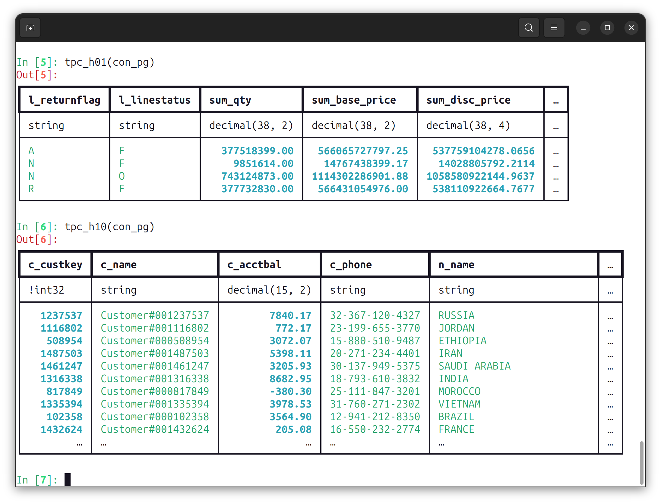
def tpc_h01(con):
    """    
    This query reports the amount of business that was billed, shipped, and returned.
    
    The Pricing Summary Report Query provides a summary pricing report for all lineitems
    shipped as of a given date. The date is within 60 - 120 days of the greatest ship date
    contained in the database. The query lists totals for extended price, discounted extended
    price, discounted extended price plus tax, average quantity, average extended
    price, and average discount. These aggregates are grouped by RETURNFLAG and LINESTATUS,
    and listed in ascending order of RETURNFLAG and LINESTATUS. A count of the number of
    lineitems in each group is included.
    """
    lineitem = con.table("lineitem")
    q = (
        lineitem
        .filter(_.l_shipdate <= (ibis.date('1998-12-01') - ibis.interval(days=90)))
        .aggregate(
            by=[_.l_returnflag, _.l_linestatus],
            sum_qty=_.l_quantity.sum(),
            sum_base_price=_.l_extendedprice.sum(),
            sum_disc_price=(_.l_extendedprice * (1 - _.l_discount)).sum(),
            sum_charge=(_.l_extendedprice * (1 - _.l_discount) * (1 + _.l_tax)).sum(),
            avg_qty=_.l_quantity.mean(),
            avg_price=_.l_extendedprice.mean(),
            avg_disc=_.l_discount.mean(),
            count_order=_.count()
        )
        .order_by([_.l_returnflag, _.l_linestatus])
    )
    return q

def tpc_h10(con):
    """
    The query identifies customers who might be having problems with the parts that are
    shipped to them.
    
    The Returned Item Reporting Query finds the top 20 customers, in terms of their effect
    on lost revenue for a given quarter, who have returned parts. The query considers only
    parts that were ordered in the specified quarter. The query lists the customer's name,
    address, nation, phone number, account balance, comment information and revenue lost.
    The customers are listed in descending order of lost revenue. Revenue lost is defined
    as sum(l_extendedprice*(1-l_discount)) for all qualifying lineitems.
    """
    lineitem = con.table('lineitem')
    orders = con.table('orders')
    customer = con.table("customer")
    nation = con.table("nation")
    
    q = (
        customer
            .join(orders, orders.o_custkey == customer.c_custkey)
            .join(lineitem, lineitem.l_orderkey == orders.o_orderkey)
            .join(nation, customer.c_nationkey == nation.n_nationkey)
    )

    q = q.filter(
        [
            (q.o_orderdate >= ibis.date("1993-10-01")) & (q.o_orderdate < (ibis.date("1993-10-01") + ibis.interval(months=3))),
            q.l_returnflag == "R",
        ]
    )

    gq = q.group_by(
        [
            q.c_custkey,
            q.c_name,
            q.c_acctbal,
            q.c_phone,
            q.n_name,
            q.c_address,
            q.c_comment,
        ]
    )
    q = gq.aggregate(revenue=(q.l_extendedprice * (1 - q.l_discount)).sum())

    q = q.order_by(ibis.desc(q.revenue))
    return q.limit(20)

Approach

For each backend we are going to test, we will first set up the connection, and call the two functions that run the TPC-H queries we want to test.

To set up the connection with Ibis, each backend uses the same pattern:

con = ibis.<name_of_backend>.connect(<parameters of the connection>)

Because Ibis uses deferred execution, to measure the actual time the queries take to compute, we need to add .execute() after our function calls to ensure that the expression is actually executed.

Postgres

With Postgres, to establish the connection using Ibis, we need to pass the name of the database, the host, and the credentials.

pg_user = os.environ.get("PG_USER")
pg_pwd = os.environ.get("PG_PWD")
con_pg = ibis.postgres.connect(database='tpc-h-10gb', host='localhost', user=pg_user, password=pg_pwd)

Once the connection is established, we can pass it to our functions and check that the outputs look as expected. In this post, we only show the output for the Postgres backend but the other backends produce the same output. Don’t be alarmed if you cannot make sense of the ‘comments’ and ‘address’ fields in the output of Q10. The data used by the TPC-H test suite is generated to have the attributes of realistic business data but some string fields are actually made up of gibberish text.

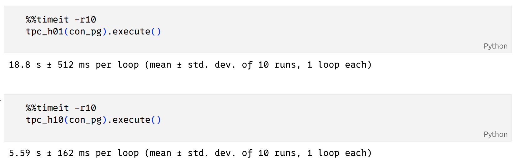
We are now ready to measure how long it takes to run our queries by running it 10 times, using the %%timeit magic:

DuckDB

To read Parquet files with the DuckDB backend, we will rely on first creating a DuckDB connection, and then registering each parquet file to it to create tables:

con_duck = ibis.duckdb.connect()
con_duck.register("/home/francois/datasets/tpc-h-10GB/parquet/lineitem.parquet", table_name="lineitem")
con_duck.register("/home/francois/datasets/tpc-h-10GB/parquet/orders.parquet", table_name="orders")
con_duck.register("/home/francois/datasets/tpc-h-10GB/parquet/customer.parquet", table_name="customer")
con_duck.register("/home/francois/datasets/tpc-h-10GB/parquet/nation.parquet", table_name="nation")
con_duck.list_tables()          

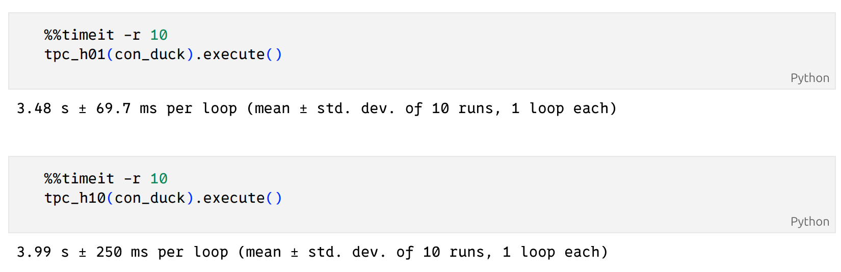
['nation', 'customer', 'orders', 'lineitem']

We can now pass the connection object directly to our functions and measure their execution time:

Spark

With Spark, we start by establishing the session as if we were using it with PySpark:

from pyspark.sql import SparkSessionspark = SparkSession.builder.config("spark.driver.memory", "25g").appName("tpc-h-10GB").getOrCreate()

We can now connect to this session with Ibis using:

con_spark = ibis.pyspark.connect(spark)

To import the data, we’ll use the register method and specify the table name, as we did for the DuckDB backend above:

con_spark.register("/home/francois/datasets/tpc-h-10GB/parquet/lineitem.parquet", table_name="lineitem")
con_spark.register("/home/francois/datasets/tpc-h-10GB/parquet/orders.parquet", table_name="orders")
con_spark.register("/home/francois/datasets/tpc-h-10GB/parquet/customer.parquet", table_name="customer")
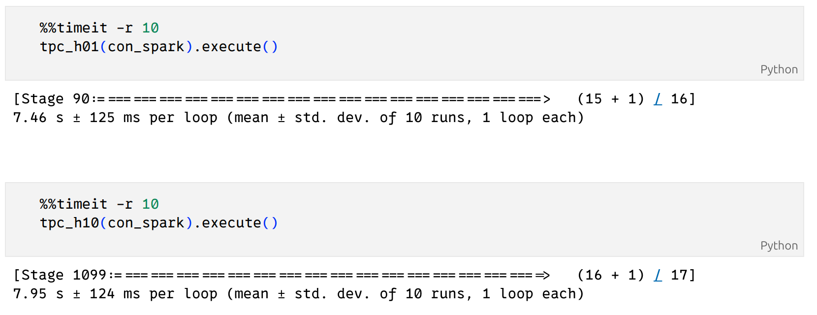
con_spark.register("/home/francois/datasets/tpc-h-10GB/parquet/nation.parquet", table_name="nation")

As with the two other backends, we can time how long it takes for these queries to run on Spark:

Results summary

In our limited tests, we found that DuckDB was the fastest for both Q1 and Q10. For Q1, Postgres took almost 5 times longer than DuckDB, and Spark took 2.5 times longer. For Q10, Postgres took 1.5 times longer than DuckDB and Spark took almost twice as much time.

Execution time for TPC-H queries 1 and 10 across 3 database engines (Postgres, Spark, and DuckDB). The point represents the mean, and the line shows the standard deviation based on 10 replicates.

Ibis helps you lower costs

In this post, we showed how Ibis can help you lower costs by helping you choose the right backend for your data needs. Ibis makes the process of testing data queries across the 18+ backends that it supports straightforward. It saves you time by writing your queries once, allowing you to test how they perform on the backends you want to evaluate.

In this example, our benchmarking with about 10 GB of data showed that DuckDB performed best overall, but Postgres closed the gap capably for Q10, and Spark performed well consistently. What does this mean for the benchmarked use case? DuckDB is single-node in-memory, is perfect to handle 10 GB, and the results reflect that. If you only need to work with about 10 GB, DuckDB is likely the right choice out of the trio.

However, having your queries written in Ibis means that if the scale of your data changes, you could easily run this test again, or a new test set, with just a few extra lines of code. Keep your query as is, and you’ll soon know exactly what backend will serve your use case for a growing and changing world.

Ibis is an open-source project and its development takes place on GitHub. The Ibis website is a great place to get started with comprehensive documentation and tutorials. If you want to explore further how Ibis can support your business needs, see how Voltron Data Enterprise Support can help you.

Resources

The code featured in this blog post is available as a Python notebook on GitHub.

Photo by Coline Beulin