GPUs for Analytics: An Experiment with Tuning, Chunking, Compression & Decompression
By
J
Joost HoozemansandK
Kae SuarezAuthor(s):
J
Joost HoozemansK
Kae SuarezPublished: September 27, 2023
10 min read
TL;DR: Graphical Processing Units (GPUs) are getting a lot of attention with the rise of generative artificial intelligence (GenAI), but that’s not all they’re good for. In this blog, we demonstrate how you can harness GPUs to accelerate data analytics workflows when working with substantially large compressed files, giving you a path toward optimized performance in both data transfer and data access.
Graphical Processing Units (GPUs) can be powerful accelerators for almost any computing system. They were designed, as their name suggests, to specialize in a certain subset of computing operations at the cost of not being as good with general computing operations. Luckily for those of us working in the data processing and artificial intelligence (AI) domains, the same subset of operations that GPUs speed up apply to a lot of the work we do as well. So with the same footprint of dozens of CPU cores, we can have thousands of specialized GPU cores working in parallel.
One emerging area where GPUs shine is data analytics. Companies like NVIDIA have built tools like CuDF to exploit massive parallelism found in GPUs for fast data analysis. With this, GPUs offer the opportunity to gain insights from your data much faster.
In this post, we’ll explore how you can augment your system to prepare for GPUs by configuring your file compression schemes to best exploit GPUs when using nvCOMP.
Compression
Data compression and decompression are long-standing components of many data workflows. Between throughput and the cost of storage, an efficient compression algorithm can save time by limiting data movement, and reduce costs by minimizing the size of files, making it a vital part of how you manage your data.
As with many algorithms, compression was originally created in a sequential, single-threaded world. As CPUs gained more cores, and distributed computing became more common, compression needed to become scalable. The most straightforward way to scale de/compression is using a technique known as “chunking.” By breaking the data to be compressed into segments, you can use those traditional but powerful sequential techniques on individual segments of data and have different processing cores handle each segment.
GPU cores are not as powerful as CPU cores individually, but the sheer number of cores found in a GPU makes up for the deficit.
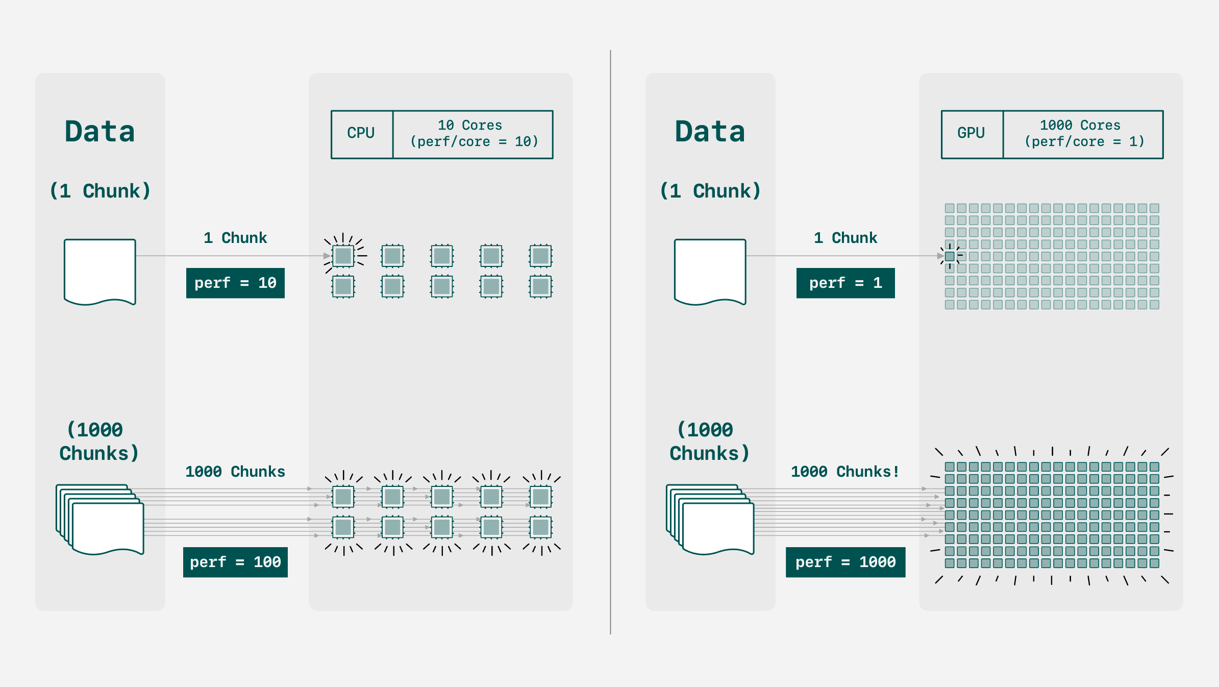
Given enough data chunks, we can leverage a GPU’s parallel nature to beat a CPU based solely on speed-to-compression. However, this chunking may negatively impact other metrics such as compression ratio, as we’ll explore here. This creates a balancing act between optimizing speed and maximizing compression ratio on GPU. Let’s explore how.
Data Chunking
Chunking goes by many names! Chunks may also be named segments, parts/partitions, batches, et cetera. It is the general technique of breaking down a problem into subsets that can be solved as their own problems, and then have their solutions concatenated
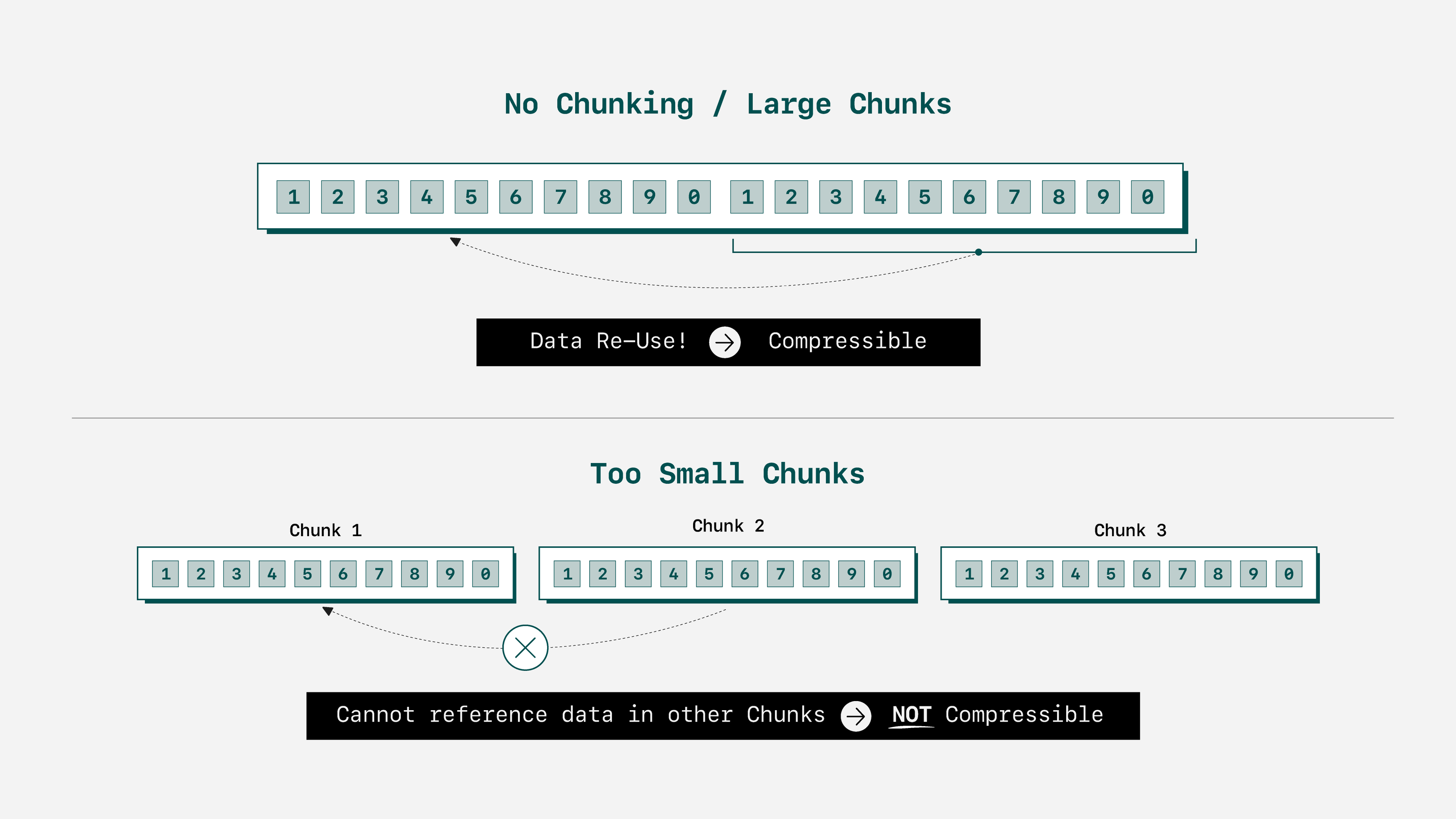
As stated, chunking is the technique that adds parallelism to compression and decompression. Compression in general is most effective when applied to large amounts of data because compression algorithms leverage patterns in the data to reduce how many bits are needed to store it. For example, little can be done to reduce abc, but abcabc can be reduced to 2abc. Since chunking divides the data into smaller sets, being too aggressive in chunking (as in the data is cut into very small pieces) can reduce the detectable patterns and thus decrease the effectiveness of compression.
Therefore, we are left to consider three possible scenarios:
- Chunk size too large/too few chunks: Compression ratio will be optimal — there’s plenty of data. However, your hardware will not be fully utilized. Five tasks running on 250 hardware threads means only five threads are used.
- Perfect chunk size/perfect chunk count: Compression ratio will be optimal or near-optimal, and throughput will be high because your hardware is fully utilized.
- Chunk size too small/too many chunks: Compression ratio will eventually decline, as the algorithm lacks patterns and trends to act upon. Throughput gains may continue, but plateauing is an inevitability. 1,000 tasks running on 250 hardware threads leverages parallelism just as well as 250 tasks on 250 threads.
With this hypothesis in mind, we can lay out our experiment.
Experiment Setup
Our goal here is to test whether a chunk size in file compression (if configured well) has a sweet spot where a GPU can perform well without sacrificing compression performance. We’ll test a variety of chunk sizes on data with some different properties, and record throughput and compression ratio.
Hardware
Our hardware platform is a bare-metal machine with:
- Intel Xeon Platinum 8380 CPU @ 2.30GHz.
- 4TB of memory (32 slots) @ 3200MHz.
- NVIDIA A100-SXM4-80GB connected via PCIe Gen4 16x.
Software + Algorithms
As mentioned previously, we’ll use nvCOMP to handle compression and decompression. This is the standard library for compression on Nvidia GPUs, so it is the clear choice for exploring performance as if in a real-world environment. The version we used is 3.0.1. As for algorithms, we’ll use:
- Snappy, a compression standard that favors high throughput over compression ratios. Very popular in the analytics space.
- zstandard (zstd), a slightly newer standard that focuses on good compression ratios but also has very good (decompression) performance.
Testing both will help us see if there is variation in how chunk size affects compression across algorithms, or if our hypothesis holds generally.
Metrics
The metrics of importance are throughput, measured in GB/s of raw data processed by the algorithm, and compression ratio, which is the ratio between the size of the original file and the compressed version.
Data
In the field of data compression, there exists a set of standard files that have various traits, called the Silesia corpus. We use data from the corpus to ensure we have a spectrum of features, thus encapsulating multiple use cases by simply including many of them.
We add an additional file in the form of data from TPC-H, already compressed and encoded as Parquet. Already-compressed data presents a difficult problem for compression — we expect a very poor ratio, but wanted to include such an edge case.
Using the above sources, we created 8GB files by repeatedly concatenating the files until they were 8GB in size.
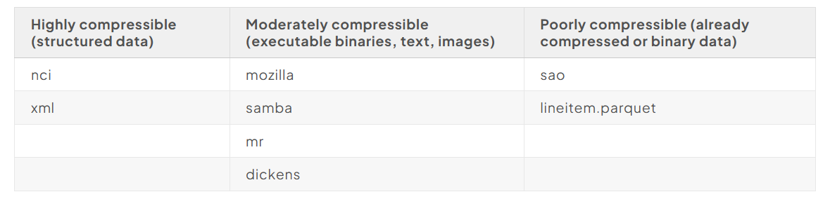
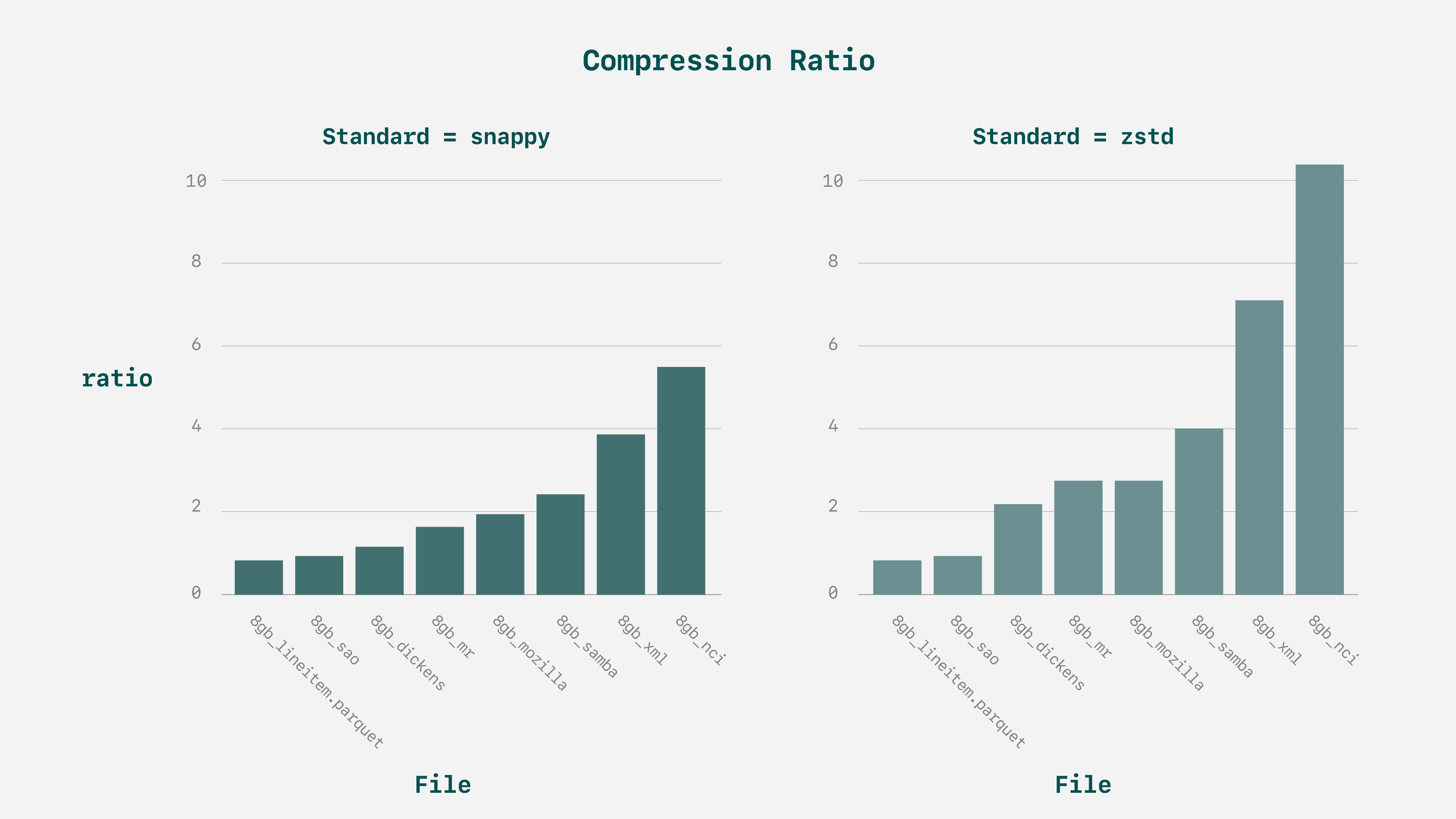
Overall, testing with default settings shows the files cover a range of compressibility:
Benchmarks
Instead of developing our own benchmark code, we use the benchmark binaries from nvCOMP, which can be used on arbitrary data. The settings can be tuned, including chunk size and algorithm, which are what we care about. Furthermore, these benchmarks automatically exclude time spent on disk read + write, so we isolate the compression and decompression throughput.
As for our exact tests, we’ll do a sweep of various chunk sizes, ranging from very large chunks that will, hypothetically, struggle on the GPU, to very small ones which should show poor compression ratio but trivially accessible parallelism. This comes out to a range of 512 to 8388608 chunks.
Experiment Outcomes
Compression Ratio
First, let’s explore at what chunk size the compression ratio starts to degrade.
Note:
For zstd, chunk sizes larger than 16M are not supported.
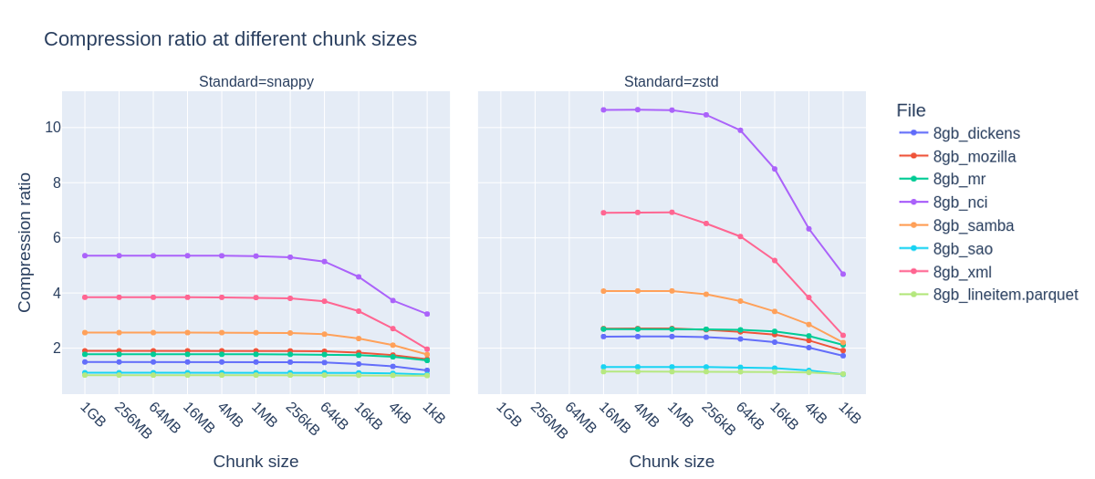
For zstd, degradation in compression ratio begins when chunk sizes reach 256 kB, while snappy sees this decline start at 64 kB. The reason for the decline in compression ratio is discussed above: small enough chunks just have less opportunity for compression. As for the different values where we see degradation, that is a trait of the algorithm. Different algorithms require different minimum amounts of data for optimal performance.
Ideally, we do not have to accept a meaningful decline in compression ratio to find better throughput. After all, it could easily be argued that the benefits of compression lie in the size on disk — not how fast you can do it. The only way to know is to test — will we be able to leverage the GPU without giving up effective compression ratios?
Compression/decompression Throughput
Note:
In the following graphs, we will include the average compression ratio across all the files for simplicity.
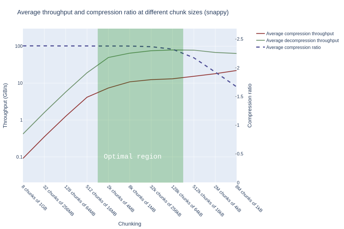
The answer is a firm “yes”. For Snappy, throughput starts slowly plateauing around 2048 chunks (chunk size 4MB) — which happens to be well before the point of degradation in compression ratio, which begins in earnest around 128k chunks (chunk size 64 kB). Decompression throughput is an order of magnitude faster than compression, but this is a trait of compression and decompression, rather than the use of a GPU.
Starting at 512k chunks (chunk size 16kB), we see another slight increase in compression throughput, but the gain is not worth the loss in compression ratio.
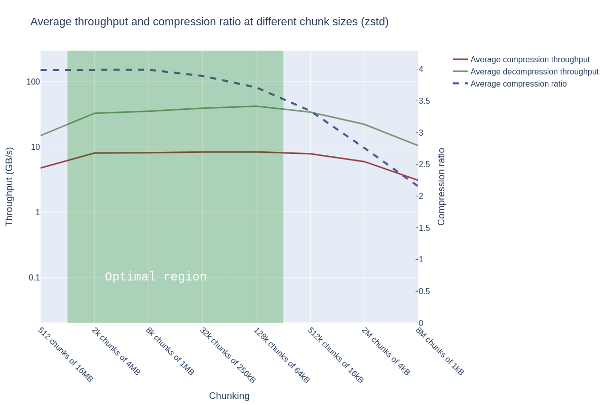
Note:
Recall that zstd has fewer data points due to its 16MB chunk size limitation.
The performance plateau spans from 2k to 512k chunks, after which performance starts to decline (which is interesting, because this behavior is opposite to Snappy!). The compression ratio starts to degrade slightly earlier than Snappy. When also taking into account the decrease in compression ratio, it seems both algorithms have an optimal region spanning from approximately 2k chunks to 128k chunks.
Why do both algorithms have an optimal region starting at 2k chunks — and why does performance stop improving afterward? The GPU excels when there are enough chunks to process — and since the A100 has approximately 7000 cores, there is a limit on how much parallelism can be exploited.
We must also note that the performance when decompressing is fantastic — and outstrips the speed of I/O (the PCIe bus here maxes out at 32 GB/s)! This performance ensures that there’s no computational bottleneck for using compressed data — just compress and enjoy the faster file reads over the bus.
Conclusion
What we learned from this experiment is that we could achieve both throughput AND high compression ratio without compromising one or the other when using a GPU. All we needed was some exploration to find the sweet spot.
Moving more parts of your pipeline to GPU ensures you spend less time moving data between CPU and GPU, and the more you leverage accelerators, your workflows will be better positioned for analytics or machine learning. Modernizing data systems means simplifying workflows: one language and one memory space, not thrashing data between APIs and hardware. I/O and compression/decompression are often delegated to CPUs, but with GPU Direct Storage and nvCOMP, you can use your GPU for ingestion with just a little tuning.
Voltron Data designs and builds data systems and pipelines to leverage the best hardware anywhere you have it — making sure everything is tuned to avoid losing any performance while doing so. To learn more about our work, check out our Product page.
Previous Article

Keep up with us